Understanding Fixed Shares
When a parent resource pool is not configured to be scalable, the shares configured for its child resource pools provide a way to prioritize allocation of fixed fractions of the parent resource pool to its children. This serves to isolate users of sibling resource pools so that virtual machines in one child resource pool cannot impact the performance of virtual machines in other child resource pools.
Suppose for example a cluster has 3 physical cores running at 2GHz, for a total of 6GHz. The root resource pool has a total of 6GHz of virtual CPU capacity to divide between its children. If there is no resource contention, all running virtual machines can be allocated their configured amounts of CPU. If there is contention for CPU resources, the 6GHz is divided between child resource pools according to the CPU shares configured for them.
This fictional data center has two child resource pools, each supporting the users in a different division of a business. Division 1 and Division 2 start out about the same size, so the IT department configures RP1 and RP2 with equal values for custom shares, and an equal number of virtual machines.
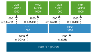
All child resource pools and virtual machines are configured with custom settings of 1000 shares each. Because the two resource pools are configured with the same number of shares, they can allocate the same amount of compute resource to their virtual machines in cases of resource contention. Likewise, all virtual machines are entitled to draw the same fraction of compute resource as their siblings.
In effect, a non-scalable resource pool guarantees that each of its children gets a fixed fraction of its resources. However, the amount allocated to each child is fixed only in relation to the quantity of resources controlled by the resource pool itself. If a root resource pool gains additional resources due to a hardware upgrade, all its children gain resource entitlements in proportion to their configured shares.
For example, suppose the cluster has been upgraded from 3 to 6 physical cores running at 2GHz, for a total of 12GHz of pooled physical capacity. The root resource pool now has a total of 12GHz of virtual CPU capacity to divide between its children. If there is contention for CPU resources, the 12GHz is divided between child resource pools according to the CPU shares configured for them.
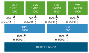
After the upgrade, each virtual machine is entitled to twice its previous resource allocation, in absolute terms. However, if another child, whether resource pool or virtual machine, is added to a parent pool, previously existing children find their resource allocation reduced, as the pool's resources are shared between more children.
Suppose Division 2 hires some new users, and IT adds an extra virtual machine to RP2 for their use.
Where previously all virtual machines in the business had the same priority for allocation of scarce compute resource, increasing the virtual machine load in RP2 means that more virtual machines contend for the same quantity of its resource. Consequently, each virtual machine in RP2 might see its performance reduced when all virtual machines are running at full capacity.
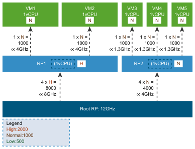
To continue from the previous example, some users in Division 1 might be concerned about performance because they plan to hire more employees in the future. Suppose they persuade the IT department that their virtual machines should be in a higher priority resource pool than others, so they will have access to more compute resource if needed. The IT department configures different custom shares values for RP1 and RP2, so that RP1 has twice the priority of RP2.
The child resource pool RP1 has 2000 shares
configured, and RP2 has 1000 shares configured, so RP1 gets 2/3 of the physical CPU
resources to share among its children, and RP2 gets 1/3 of the physical CPU resources to
share among its children. You can calculate the amount of compute resource available to
RP1 for its children as 12 x 2000 / (2000+1000) = 8GHz, and the amount
of compute resource available to RP2 for its children as 12 x 1000 / (2000+1000)
= 4 virtual GHz. The children within each resource pool have identical
shares settings, so they share their own pool's resources equally.
Now suppose a new CIO joins the business and decides that from now on priority shares should be specified as levels rather than custom values. The IT department reconfigures all the shares settings to use the enums for shares levels.
When you specify shares levels, you have to make two calculations. First you convert the specified level to a numeric value that corresponds to custom shares settings. This conversion takes into account the number of virtual cores.
Then you use that numeric value to calculate the proportion of resources to allocate to the child pool, in the same way as with the custom shares settings.
To convert a shares level to a numeric value,
multiply the number of vCPUs by a constant that corresponds to the level. For the
purpose of this calculation, all resource pools have an implicit size of 4 vCPUs. Use
the VirtualMachine.config.hardware.numCPU value as the number of vCPUs
for virtual machines. The constant for the high priority level is 2000,
and the constant for the normal level is 1000. You can calculate that
the numeric shares belonging to RP1 are 4 x 2000 = 8000. RP2 has a
priority level of normal, so the numeric shares belonging to RP2 are
4 x 1000 = 4000. The compute resource that RP1 can allocate is
12 x 8000 / (8000+4000) = 8 GHz, and the compute resource that RP2
can allocate to its children is 12 x 4000 / (8000+4000) = 4 GHz. The
new CIO is satisfied that RP1 and RP2 achieve the same result with priority levels as
with the previous custom shares values.
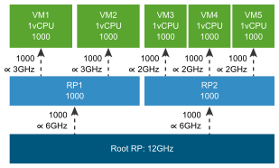
But suppose the IT department is asked to support a 3rd division, newly acquired by the business, which is about the same size as the division assigned to RP2. The IT department creates a new child resource pool, RP3, and configures the same number of virtual machines and the same shares levels as RP2. Now the division of resources looks like this:
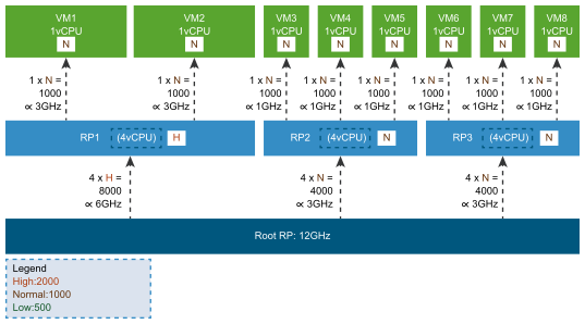
Assume the hardware resources available to the root resource pool have not changed at the time of the acquisition, so the 12GHz of virtual compute resource must be divided into fractions according to the configured shares of the child resource pools. After adding RP3, both RP1 and RP2 get less of the virtual compute resource to divide among their own children.
Virtual machines available to Division 1 now
compete for 12 x 8000 / (8000+4000+4000) = 6GHz in RP1. Virtual
machines available to Division 2 compete for 12 x 4000 / (8000+4000+4000) =
3GHz in RP2. Virtual machines available to Division 3 similarly compete for
12 x 4000 / (8000+4000+4000) =
                3
GHz in RP3.
In this example, Division 1 and Division 2 employees might both perceive reduced performance until the IT department's capital budget increases to support the new configuration.
When Division 1 hires a number of new
employees, IT adds two more virtual machines to RP1 to accommodate the increased size of
Division 1. All four virtual machines in RP1 still benefit from RP1's
high priority level, but now that RP1's compute resources are
spread among a larger number of virtual machines, each of its virtual machines gets a
smaller allocation when they are competing for CPU cycles.
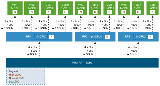
Some virtual machine users who were in
Division 1 before the new employees joined are noticing greatly reduced performance.
They are only getting 1.5GHz where they used to get 3GHz. When they learn that Division
2 employees are getting 1GHz from their virtual machines in RP2, which has
normal priority, they might not be happy that they are getting only
1.5GHz from virtual machines in RP1, which has high priority.
The disappointed users speak to the IT department, where they learn that this is the way fixed shares for resource pools are intended to work. They isolate Division 1 virtual machine performance from the other divisions, but not from other users of the same resource pool. These Division 1 users learn that there are other ways to protect the performance of high priority virtual machines.
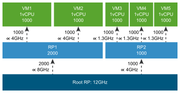
Some Division 1 users try other ways to get more compute resource from RP1's fixed allocation. They request changes to virtual machine configurations, which result in increased priority for some of their virtual machines at the expense of others.
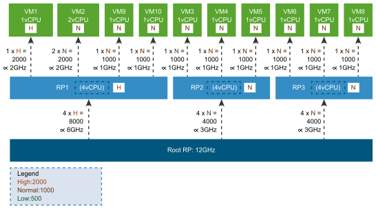
After VM1 is reconfigured, you calculate its numeric shares by multiplying the configured
numCPU (1) by its shares level (high), getting
1 x 2000 = 2000. You calculate its resource allocation by using its
numeric shares to prorate the allocation available to its parent resource pool:
6GHz x 2000 /
                (2x2000+2x1000) = 2GHz
.
You calculate VM2's numeric shares by multiplying the configured numCPU
(2) by its shares level (normal), getting 2 x 1000 =
2000. You calculate its resource allocation by using its numeric shares to
prorate the allocation available to its parent resource pool: 6GHz x 2000 /
(2x2000+2x1000) = 2GHz.
In a similar way, calculate VM9's numeric shares by multiplying its configured
numCPU (1) by its shares level (normal), getting
1 x 1000 = 1000. You calculate its resource allocation by using its
numeric shares to prorate the allocation available to its parent resource pool:
6GHz x 1000 / (2x2000+2x1000) = 1GHz. VM10's resource configuration
and associated calculations are identical to VM9.
When other Division 1 users realize that VM9 and VM10 only get 1GHz of virtual compute
resource, they might not be satisfied with this result. These virtual machines are in a
high priority resource pool, but they get the same resource
allocation as Division 2's virtual machines, which are in a normal
priority resource pool. That doesn't seem fair.
Division 1 users request a meeting with the CIO, who explains that the scalable shares feature is the best solution to their problem.